Computational Fluid Dynamics for fans and plants
1 / 16Pages

Innovations from Venti Oelde Computational Fluid Dynamics for fans and plants

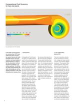
Computational Fluid Dynamics for fans and plants Fan optimization with CFD modelling In the field of turbomachinery construction, CFD has, within the space of just a few years, become an indispensable tool for the optimization and new design of turbomachines, as well as for the elimination of fluidmechanic problems in installed systems. The following paper demonstrates the basic knowledge as well as applied examples of the CFD simulations of process fans. Computational Fluid Dynamics (CFD) is a method that is used for the computerized calculation of technical flows with state-of-the-art...

(nodes). In this way, the continuous distribution of Φ is represented by the Φ values at discrete points. This creates an algebraic equation (finite difference equation) for every calculation point representing a single computation volume (cell). This algebraic equation is then used for determining the flow values. The differential equations from all the calculation points form a system of linked algebraic equations. This system of equations has to be solved with a numeric algorithm. A number of direct or iterative calculation methods are available for the solution of algebraic equation...

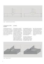
Figure 1 Parameterized layout with modification To allow performance of a CFD simulation a number of work steps have to be carried out in the sequence described below. It is presumed for this purpose that the geometry data and the boundary conditions are known: The first step is to create a three-dimensional model of the geometry using CAD software with 3D capability. It must be remembered at this stage that in the case of flow simulations the 3D geometry of the flow zone is needed and not that of the structure, as is usual in other types of analysis. Increasingly, the created 3D models are...

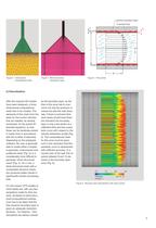
Laminar boundary layer Turbulent flow w Figure 3 Unstructured computational mesh Figure 4 Block-structured hexahedral mesh Figure 5 Flow profile After the required 3D models have been designed, a threedimensional computational mesh has to be created. The elements of this mesh form the basis for the control volumes that are needed, as already mentioned, for the partial differential equations, so that these can be iteratively solved in matrix form in accordance with the number of elements. Depending on the employed software, the user is generally able to create either a simpleto-generate,...

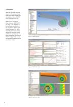
c) Simulation After the 3D model and subsequently the computational mesh have been created, the simulation software (ANSYS CFX) is brought into use. ANSYS CFX consists of three modules: ANSYS CFXPre (Fig. 7) for definition of the boundary conditions of the simulation, ANSYS CFX Solver Manager (Fig. 8) for iteratively solving the partial differential equations until a predefined convergence criterion is reached, and ANSYS CFX Post (Fig. 9) for visual and numeric evaluation of the simulation results. Figure 7 ANSYS CFX-Pre Figure 8 ANSYS CFX Solver Figure 9 ANSYS CFX Post

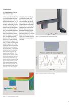
4 Applications 4.1 Optimization of the intake flow of a stack ent coming from the left was considerably higher than that entering the collecting duct from below. As can be clearly seen from Fig. 11, this causes a severe constriction of the air stream entering the collecting duct from the bottom left. As a consequence, there were pressure fluctuations in excess of 250 Pa in this supply duct (Fig. 12), and these throttled the fan so severely that it reacted with significantly increased vibration velocities. Figure 10 Stack geometry with marked problem zone Pressure gradient at measuring...

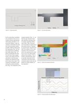
Figure 13 Original geometry As the described unsatisfactory conditions had to be remedied without significantly interrupting operation or altering the design, it was necessary to eliminate the problem by the simplest means possible. Without altering the duct geometry (Fig. 13), this was achieved by installing two baffle plates (Fig. 14), which accelerated the flow from the two lower supply ducts to the extent that the velocities of all three gas streams are identical at the point where they meet. This measure succeeded in optimizing the velocity distribution (Fig. 15) compared to the Figure...

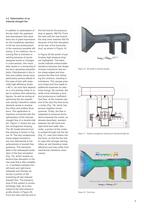
4.2 Optimization of an induced draught fan In addition to optimization of the fan itself, the upstream and downstream flow situations are of great importance for the troublefree operation of the fan and achievement of the maximum possible efficiency. If, for instance, the incoming flow is turbulent or swirling because of poorly designed bends or changes in cross-section, this inevitably results in a worsening of the fan’s operating characteristics. Disturbances in the inflow and outflow zones have particularly serious effects in the case of fans with especially high efficiency levels > 80...

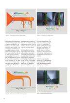
Pressure loss outlet 1 = 261.365 [Pa] 0 Pressure loss outlet 1 = 261.365 [Pa] Pressure loss outlet 2 = 431.966 [Pa] Pressure loss outlet 2 = 431.966 [Pa] 30 Optimization of the geometry involved redesigning the critical points highlighted in Fig. 20 so that the cross-section transitions were smooth. This redesigning succeeded in reducing the pressure drop at the front inflow duct to the fan by a factor of four, from 261 Pa to 66 Pa (Fig. 22), while the pressure drop at the rear inflow duct that had been caused by the poorly-designed horizontal duct end (Fig. 20, white circle) was even...

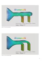
Pressure loss outlet 1 = 261.365 [Pa] Pressure loss outlet 2 = 431.966 [Pa] Figure 24 Flow lines of original design Pressure loss outlet 1 = 65.8793 [ Pa ] Pressure loss outlet 2 = 76.8992 [Pa] Figure 25 Flow lines of optimized design

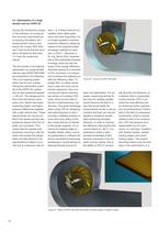
4.3 Optimization of a large double-inlet fan DHRV 50 During the introduction phase of the software, its computation accuracy was tested by comparing simulation and measurement using a testbench fan of type HRV 63S and it was found that the simulation deviated by less than 1% from the measured values. The first results of an ongoing optimisation of a large doubleinlet fan type DHRV 50B-2000 are presented in the following. This is an ongoing project which has the aim of determining the optimization potential of the DHRV 50, particularly at high peripheral speeds > 150 m/s. The background to...