
- Catalogs
- Siglent Technologies Co., Ltd
- Siglent Spectrum Analyzer SSA3000X Series DataSheet

- Company
- Products
- Catalogs
- News & Trends
- Exhibitions
Siglent Spectrum Analyzer SSA3000X Series DataSheet

Siglent Spectrum Analyzer SSA3000X Series DataSheet
The SSA3000X Series Spectrum Analyzer supports remote control via USB and LAN interfaces using NI-VISA and programming languages. Communication can be established using VXI-11, Sockets, and Telnet protocols.
1.1 Build Communication
Using VISA: Install NI-VISA, connect the spectrum analyzer to the PC via USB, and follow installation prompts.
Using Sockets: Use TCP/IP over LAN with standard mode on port 5025 and Telnet mode on port 5024.
1.2 Remote Control Capabilities
Users can program the analyzer using SCPI commands and control it via NI-MAX software.
SCPI Overview
SCPI commands are structured hierarchically with root and subkeywords. Commands start with ":" and parameters follow a space. Queries end with "?".
2.1 Command Format
Commands are structured with root and subkeywords, separated by colons. Parameters follow a space, and queries end with a question mark.
2.2 Symbol Instruction
Symbols like <>, [], |, and {} are used for parameters but not sent with commands.
2.3 Parameter Type
Parameters include boolean, enumeration, integer, float, discrete, and string types.
2.4 Command Abbreviation
Commands are case-insensitive, but abbreviations must include all capital letters.
System Commands
This section details SCPI commands for various subsystems, including IEEE Common Commands, System, Instrument, Initiate, Sense, Calculate, Measurement, Trigger, TG, Demod, and Calibration subsystems.
3.1 IEEE Common Commands
Includes commands like *IDN? for identification, *RST for reset, *CLS for clearing status, and *OPC? for operation complete queries.
3.2 System Subsystem
Commands for setting system time, date, IP address, and gateway are provided, with examples for each.
- Gateway: Automatically fetched if IP assignment is set to DHCP. Command:
:SYSTem:COMMunicate:LAN:GATeway. Example::SYSTem:COMMunicate:LAN:GATeway "192.168.1.1". - Subnet Mask: Set according to PC network settings, automatically if DHCP. Command:
:SYSTem:COMMunicate:LAN:SMASk. - IP Config: Toggle between static and DHCP. Command:
:SYSTem:COMMunicate:LAN:TYPE. Example::SYSTem:COMMunicate:LAN:TYPE DHCP.
- Language: Set to Chinese or English. Command:
:SYSTem:LANGuage. Example::SYSTem:LANGuage SCHINESE. - Power On Type: Set to default, last, or user state. Command:
:SYSTem:PON:TYPE. Example:SYSTem:PON:TYPE DFT. - System Preset: Preset instrument based on preset type. Command:
:SYSTem:PRESet. - System Restart: Restart the instrument. Command:
:SYSTem:RESTart. - Factory Reset: Reset to factory settings. Command:
:SYSTem:FDEFault. - Enable Option: Enable options with a license key. Command:
:SYSTem:LKEY. - Installed Options Query: List installed options. Command:
:SYSTem:OPTions?. - Power Off: Turn off the instrument. Command:
:SYSTem:POWer:OFF. - System Info: Query system message. Command:
:SYSTem:CONFigure:SYSTem?.
- Instrument Mode: Set to Spec Analyzer or Reflection Meas. Command:
:INSTrument[:SELect]. - Measure Mode: Set various measurement modes. Command:
:INSTrument:MEASure.
- Single Sweep: Set single sweep. Command:
:INITiate[:IMMediate]. - Continuous or Single Sweep: Toggle sweep mode. Command:
:INITiate:CONTinuous.
- Frequency Subsection: Set center, start, stop frequencies, and span. Commands include
[:SENSe]:FREQuency:CENTer,[:SENSe]:FREQuency:STARt,[:SENSe]:FREQuency:STOP, and[:SENSe]:FREQuency:SPAN. - Auto Tune: Auto tune the spectrum analyzer. Command:
[:SENSe]:FREQuency:TUNE:IMMediate. - Amplitude Subsection: Set reference level, input attenuator, preamp state, and amplitude units. Commands include
:DISPlay:WINDow:TRACe:Y[:SCALe]:RLEVeland[:SENSe]:POWer[:RF]:ATTenuation.
- Grid Brightness: The command
:DISPlay:WINDow:TRACe:GRATicule:GRID:BRIGhtness <value>sets the grid brightness, with a range from 0 to 100 and a default of 30%. The current brightness can be queried using:DISPlay:WINDow:TRACe:GRATicule:GRID:BRIGhtness?. - Display Line On/Off: The command
:DISPlay:WINDow:TRACe:Y:DLINe:STATe OFF|ON|0|1toggles the display line state, with a default of OFF. The state can be queried with:DISPlay:WINDow:TRACe:Y:DLINe:STATe?. - Display Line Amplitude: The command
:DISPlay:WINDow:TRACe:Y:DLINe <value>sets the amplitude value for the display line, with a range from the reference level to 100 dBm below it, defaulting to 0 dBm.
- Marker On/Off: The command
:CALCulate:MARKer[1]|2|3|4:STATe OFF|ON|0|1toggles the marker status, with a default of OFF. The state can be queried with:CALCulate:MARKer[1]|2|3|4:STATe?. - Marker Mode: The command
:CALCulate:MARKer[1]|2|3|4:MODE POSition|DELTa|BAND|OFFselects the marker type, with a default of OFF. The mode can be queried with:CALCulate:MARKer[1]|2|3|4:MODE?. - Marker to Trace: The command
:CALCulate:MARKer[1]|2|3|4:TRACe 1|2|3|4assigns a marker to a specific trace, defaulting to trace 1. - Marker X Value: The command
:CALCulate:MARKer[1]|2|3|4:X <para>positions the marker on its trace at a specified X value, with a range of 0 Hz to 3.2 GHz or 10 ms to 1000 s. - Reference Marker X Value: The command
:CALCulate:MARKer[1]|2|3|4:X:REFerence <para>positions the reference marker on its trace at a specified X value, used in DELTa|BAND modes. - Marker Delta X Value: The command
:CALCulate:MARKer[1]|2|3|4:X:DELTa <para>positions the delta marker on its trace at a specified X value, used in DELTa|BAND modes. - Center Pair Marker X Value: The command
:CALCulate:MARKer[1]|2|3|4:X:CENTer <para>sets the center frequency of the center pair marker, used in DELTa|BAND modes. - Span Pair Marker X Value: The command
:CALCulate:MARKer[1]|2|3|4:X:SPAN <para>sets the X value for the span of the Span Pair marker, used in DELTa|BAND modes. - Query Marker Y Value: The command
:CALCulate:MARKer[1]|2|3|4:Y?reads the current Y value for the designated marker. - Reference Marker Y Value: The command
:CALCulate:MARKer[1]|2|3|4:Y:REFerence?gets the current Y value for the designated reference marker, used in DELTa|BAND modes. - Marker Delta Y Value: The command
:CALCulate:MARKer[1]|2|3|4:Y:DELTa?gets the current Y value for the designated delta marker, used in DELTa|BAND modes. - Marker Table: The command
:CALCulate:MARKer:TABLe ON|OFF|0|1toggles the marker table status, defaulting to OFF. - Marker to Start/Stop/Center Frequency: Commands like
:CALCulate:MARKer[1]|2|3|4[:SET]:START,:STOP, and:CENTerset the start, stop, or center frequency to the marker frequency, not available in zero span. - Marker Delta to Span/Center Frequency: Commands like
:CALCulate:MARKer[1]|2|3|4:DELTa[:SET]:SPANand:CENTerset the span or center frequency to the delta marker frequency, used in DELTa|BAND modes. - Peak Search Type: The command
:CALCulate:MARKer:PEAK:SEARch:MODE MAXimum|MINimumconfigures the peak search type, defaulting to MAXimum.
Specifies the minimum signal level for peak identification. The range is -200.0 dBm to 200.0 dBm, with a default of -160.0 dBm. Example command:
:CALCulate:MARKer:PEAK:THReshold -50.Defines the minimum signal excursion above the threshold for peak recognition. The range is 0 to 200.0 dB, with a default of 0 dB. Example command:
:CALCulate:MARKer:PEAK:EXCursion 10.Toggles the peak table on or off. Example command:
:CALCulate:MARKer:PEAK:TABLe ON.Enables or disables continuous peak search. Example command:
:CALCulate:MARKer1:CPEak ON.Performs a peak search based on mode settings. Example command:
:CALCulate:MARKer4:MAXimum.Commands for starting, stopping, and querying limit tests. Example command to start:
:CALCulate:LLINe:TEST:STARt.Sets or queries the state of limit lines. Example command:
:CALCulate:LLINe1:STATe OFF.Commands for setting bandwidth and querying power in main and adjacent channels. Example command for main channel bandwidth:
:ACPRatio:BWIDth:INTegration 20 MHz.- Lower ACPR: Command
:MEASure:ACPRatio:LOWer?returns the lower adjacent channel power to main channel power ratio in dBm. - Upper ACPR: Commands
:MEASure:ACPRatio:UPPer:POWer?and:MEASure:ACPRatio:UPPer?return the upper adjacent channel power and its ratio to the main channel power, respectively.
- Integration Bandwidth: Command
[:SENSe]:CHPower:BWIDth:INTegrationsets or queries the integration bandwidth for power calculation, ranging from 100 Hz to 3.2 GHz. - Channel Span: Command
[:SENSe]:CHPower:FREQuency:SPAN:POWersets the analyzer span for channel power measurement. - Power and Density: Commands
:MEASure:CHPower?,:MEASure:CHPower:CHPower?, and:MEASure:CHPower:DENSity?return channel power and power spectral density in dBm and dBm/Hz, respectively.
- Method Selection: Command
[:SENSe]:OBWidth:METHodtoggles between percent and dBc methods for OBW measurement. - Percentage and dBc Methods: Commands
[:SENSe]:OBWidth:PERCentand[:SENSe]:OBWidth:XDBset the percentage of signal power and dBc value for emission bandwidth determination. - OBW Queries: Commands
:MEASure:OBWidth?,:MEASure:OBWidth:OBWidth?, and:MEASure:OBWidth:CENTroid?query the occupied bandwidth and centroid.
- Frequency and Limits: Commands
[:SENSe]:TPOWer:FREQuency:CENTer,[:SENSe]:TPOWer:LLIMit, and[:SENSe]:TPOWer:RLIMitset or query the T-power center frequency, start, and stop lines. - T-power Query: Command
:MEASure:TPOWer?returns the T-power measurement result in dBm.
- Spectrogram State: Command
[:SENSe]:SPECtrogram:STATesets or queries the spectrogram state (RUN or PAUSE). - Spectrogram Restart: Command
[:SENSe]:SPECtrogram:RESTartrestarts the spectrogram.
- TOI Queries: Commands
:MEASure:TOI?and:MEASure:TOI:IP3?return the TOI result and the minimum intercept of the lower and upper TOI.
- Trigger Type: Command
:TRIGger[:SEQuence]:SOURcespecifies the trigger source (IMMediate, VIDeo, EXTernal). - Video Trigger Level: Command
:TRIGger[:SEQuence]:VIDeo:LEVelsets or queries the video trigger level. - Trigger Edge: Command
:TRIGger[:SEQuence]:RFBurst:SLOPesets the trigger edge (POSitive or NEGative).
- TG On-off and Level: Commands
:OUTPut[:STATe]and:SOURce:POWer[:LEVel][:IMMediate][:AMPLitude]control the TG state and level. - Normalization: Commands
:CALCulate:NTData[:STATe]and:DISPlay:WINDow:TRACe:Y[:SCALe]:NRLevelmanage TG normalization settings.
- Demod Mode and Time: Commands
[:SENSe]:DEModand[:SENSe]:DEMod:TIMEset or query the demodulation mode and time. - Earphone and Volume: Commands
[:SENSe]:DEMod:EPHoneand[:SENSe]:DEMod:VOLumecontrol earphone state and volume.
- Calibration State: Command
[:SENSe]:CALibration:STATesets or queries the calibration state.
- Store File (:MMEMory:STORe): This command allows storing files in various formats such as STA, TRC, COR, CSV, LIM, JPG, BMP, and PNG. The command format is
:MMEMory:STORe <type>,<file>. Example::MMEMory:STORe STA,ABC.sta. - Load File (:MMEMory:LOAD): This command is used to load files of types STA, TRC, COR, and LIM. The command format is
:MMEMory:LOAD <type>,<file>. Example::MMEMory:LOAD STA,ABC.sta. - Delete File (:MMEMory:DELete): This command deletes a specified file or folder. The command format is
:MMEMory:DELete <file>. Example::MMEMory:DELete ABC.sta.
- Using VISA with VC++: The example demonstrates controlling a device using NI-VISA with USBTMC or TCP/IP access. It involves setting up a Visual Studio project, including necessary libraries, and writing functions for USBTMC and TCP/IP communication.
- Using VISA with Visual Basic: Similar to the VC++ example, this involves setting up a Visual Basic project, adding necessary libraries, and writing functions for USBTMC and TCP/IP communication.
- Using VISA with MATLAB: This example shows how to use MATLAB to control a device via USBTMC or TCP/IP using NI-VISA. It involves creating VISA objects, sending commands, and reading responses.
- Using VISA with LabVIEW: Although not detailed in the provided text, this section likely covers using LabVIEW to control devices using NI-VISA.
This document provides a guide on using LabVIEW and Python for programming and communicating with devices, specifically focusing on VISA sessions and socket programming.
LabVIEW Programming Steps
1. Open LabVIEW and create a VI file.
2. Add controls such as VISA resource name, error in, error out, and indicators in the Front Panel interface.
3. In the Block Diagram interface, add functions like VISA Write, VISA Read, VISA Open, and VISA Close from the VISA Palette.
4. Connect these functions as illustrated in the guide.
5. Select the device resource from the VISA Resource Name list box and run the program. This setup opens a VISA session to a USBTMC device, sends a command, and reads the response.
6. For TCP/IP communication, change VISA Write and Read functions to Synchronous I/O by selecting Synchronous I/O Mod from the shortcut menu.
7. Connect the functions as shown in the guide and input the IP address to run the program.
Python Socket Programming Example
This section provides an example of using Python for socket programming to communicate with devices.
Environment
- Operating System: Windows 7 32-bit
- Python Version: 2.7.5
Functionality
The Python script opens a socket, sends a query, and closes the socket in a loop 10 times.
Python Script Overview
- Import necessary modules: socket, sys, and time.
- Define the remote IP and port number.
- Create functions for connecting to the socket, sending queries, and closing the socket.
- The main function sends the SCPI command *IDN? 10 times and prints the response.
Conclusion
This guide provides step-by-step instructions for setting up communication with devices using LabVIEW and Python, highlighting the importance of configuring VISA sessions and socket connections correctly.
Catalog excerpts
Programming Guide SSA3000X Series Spectrum Analyzer
Open the catalog to page 1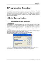
1.Programming Overview SSA3000X Series Spectrum Analyzer support both USB and LAN interfaces. By using these interfaces, in combination with NI-VISA and programming languages, users can remotely control the spectrum analyzer. Through LAN interface, VXI-11, Sockets and Telnet protocols can be used to communicate with the spectrum analyzer. This chapter introduces how to build communication between the spectrum analyzer and the PC. It also introduces the remote control capabilities. Build Communication Using VISA 1、Install NI-VISA Before programming, you need to install NI-VISA, which you can download...
Open the catalog to page 3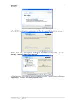
c.The NI-VISA installing dialog is shown above. Click Next to start the installation process. Set the install path, default path is “C:\Program Files\National Instruments\” , you can change it. Click Next, dialog shown as above. d. Click Next twice, in the License Agreement dialog, select the “ I accept the above 2 License Agreement(s).” ,and click Next, dialog shown as below:
Open the catalog to page 4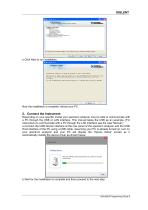
e. Click Next to run installation. Now the installation is complete, reboot your PC. 2、Connect the Instrument Depending on your specific model your spectrum analyzer may be able to communicate with a PC through the USB or LAN interface. This manual takes the USB as an example. (For instructions to communicate with a PC through the LAN interface see the User Manual.) a. Connect the USB Device interface at the rear panel of the spectrum analyzer and the USB Host interface of the PC using a USB cable. Assuming your PC is already turned on, turn on your spectrum analyzer and your PC will display...
Open the catalog to page 5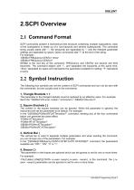
SCPI commands present a hierarchical tree structure containing multiple subsystems, each of the subsystems is made up of a root keyword and several subkeywords. The command string usually starts with “:”, the keywords are separated by “:” and the followed parameter settings are separated by space. Query commands add “?” at the end of the string. For example: :SENSe:FREQuency:CENTer <freq> :SENSe:FREQuency:CENTer? SENSe is the root key of the command, FREQuency and CENTer are second and third keywords. The command begins with “:”, and separates the keywords at the same time, <freq> separated by...
Open the catalog to page 7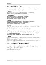
All of the commands are not case sensitive, so you can use any of them. But if abbreviation is used, all the capital letters in the command must be written completely. For example: :DISPlay:WINDow:TRACe:Y:DLINe:STATe? Can be abbreviated to: :DISP:WIND:TRAC:Y:DLIN:STAT?
Open the catalog to page 8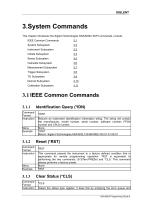
This chapter introduces the Siglent Technologies SSA3000X SCPI commands, include: IEEE Common Commands 3.1
Open the catalog to page 9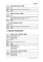
3.1.8 Status Byte Query (*STB)
Open the catalog to page 11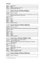
3.2.12 Factory ReSet (:SYSTem:FDEFault) Command Format
Open the catalog to page 14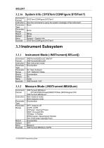
SIGLENT 3.2.16 System Info (:SYSTem:CONFigure:SYSTem?)
Open the catalog to page 16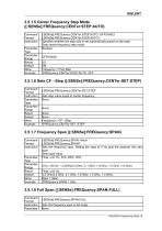
3.5.1.5 Center Frequency Step Mode ([:SENSe]:FREQuency:CENTer:STEP:AUTO)
Open the catalog to page 19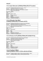
3.5.3.2 Input Attenuator ([:SENSe]:POWer[:RF]:ATTenuation) Command :DISPlay:WINDow:TRACe:Y:SCALe:RLEVel:OFFSet <value> Format |:DISPlay:WINDow:TRACe:Y:SCAI_e:RLEVel:OFFSet?
Open the catalog to page 22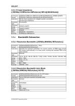
SIGLENT 3.5.3.15 Input Impedance ([:SENSe]:CORRection:IMPedance[:INPut][:MAGNitude])
Open the catalog to page 26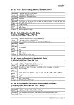
3.5.4.3 Video Bandwidth ([:SENSe]:BWIDth:VIDeo)
Open the catalog to page 27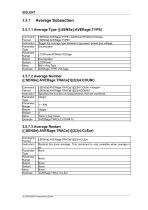
3.5.7.1 Average Type ([:SENSe]:AVERage:TYPE)
Open the catalog to page 32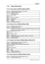
3.5.8.1 Sweep Mode ([:SENSe]:SWEep:MODE) 3.5.8.4 Sweep Speed ([:SENSe]:SWEep:SPEed) Command [:SENSe]:SWEep:SPEed NORMal|ACCUracy Format |[:SENSe]:SWEep:SPEed?
Open the catalog to page 33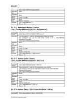
3.6.1.14 Marker Table (:CALCulate:MARKer:TABLe) Command |:CALCulate:MARKer:TABLe ON|OFF|0|1 40 SSA3000X Programming Guide
Open the catalog to page 40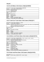
3.6.2.9 Add Limit Point Data (:CALCulate:LLINe[1]|2:DATA) Command Format
Open the catalog to page 50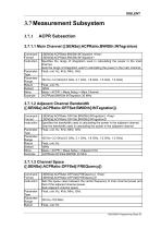
3.7.1.1 Main Channel ([:SENSe]:ACPRatio:BWIDth:INTegration)
Open the catalog to page 53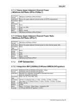
3.7.1.7 Query Upper Adjacent Channel Power (:MEASure:ACPRatio:UPPer:POWer?)
Open the catalog to page 55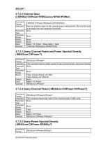
3.7.2.5 Query Power Spectral Density (:MEASure:CHPower:DENSity?) Command Format
Open the catalog to page 56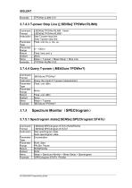
Example |:TPOWer:LLIMit 0.01 3.7.4.3 T-power Stop Line ([:SENSe]:TPOWer:RLIMit)
Open the catalog to page 60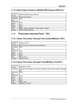
3.7.5.2 Spectrogram Restart ([:SENSe]:SPECtrogram:RESTart)
Open the catalog to page 61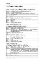
3.8.1 Trigger Type (:TRIGger[:SEQuence]:SOURce)
Open the catalog to page 62
3.9.4 TG Normalize on-off (:CALCulate:NTData[:STATe]) 3.9.7 TG Normalize Reference Trace on-off (:DISPlay:WINDow:NTTRace[:STATe]) Command | |:DISPlay:WINDow:NTTRace[:STATel OFF|ON|0|1
Open the catalog to page 64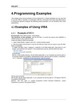
4.Programming Examples This chapter gives some examples for the programmer. In these examples you can see how to use the VISA or sockets, in combination with the commands have been described above to control the spectrum analyzer. By following these examples, you can develop many more applications. 4.1 Examples of Using VISA 4.1.1 Environment: Win7 32bit system, Visual Studio The functions of this example: use the NI-VISA, to control the device with USBTMC or TCP/IP access to do a write and read. Follow the steps to finish the example: 1、 Open Visual Studio, create a new VC++ win32 console project....
Open the catalog to page 68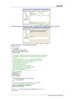
#include <visa.h> 3n Add codes: (1)USBTMC access code. Write a function Usbtmc_test: int Usbtmc_test() { /* This code demonstrates sending synchronous read & write commands */ /* to an USB Test & Measurement Class (USBTMC) instrument using */ /* NI-VISA */ /* The example writes the "*IDN?\n" string to all the USBTMC */ /* devices connected to the system and attempts to read back */ /* results using the write and read functions. */ /* The general flow of the code is */ /* Open Resource Manager */ /* Open VISA Session to an Instrument */ /* Write the Identification Query Using viPrintf */ /*...
Open the catalog to page 69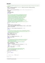
/* Find all the USB TMC VISA resources in our system and store the number of resources in the system in numlnstrs.*/ status = viFindRsrc (defaultRM, "USB?*INSTR", &findList, &numInstrs, instrResourceString); if (status<VI_SUCCESS) { printf ("An error occurred while finding resources. \nPress ’Enter’ to continue."); fflush(stdin); getchar(); viClose (defaultRM); returnstatus; } /** Now we will open VISA sessions to all USB TMC instruments. * We must use the handle from viOpenDefaultRM and we must * also use a string that indicates which instrument to open. This * is called the instrument descriptor....
Open the catalog to page 70All Siglent Technologies Co., Ltd catalogs and technical brochures
 SDS6000A Series
21 Pages
 SDS 7000A Series
21 Pages
 SDL1000X Series
10 Pages
 SSM5000A Series
15 Pages
 Spectrum Analyzer Bandwidth
6 Pages
 Siglent_Product Catalog 2016
48 Pages
 Siglent Selection Guide 2016
10 Pages
 Benefits of deep memory
3 Pages
 SIGLENT Probes Datasheet
7 Pages
 Siglent SDS2000X User Manual
197 Pages
 Siglent SDS2000X Service Manual
59 Pages
 Probe Data Sheet + Siglent
7 Pages
 USB-GPIB User Manual_Siglent
13 Pages
 ISFE User Manual
12 Pages
 Siglent TrueArb Technology
9 Pages
 SDS2000 VS DS2000A_EN_Siglent
10 Pages
 SIGLENT SDS1000CFL
8 Pages
 SIGLENT SHS800 Data Sheet
10 Pages


- Power supply unit
- DC power supply
- AC/DC power supply
- Automation software solution
- Monitoring analyzer
- Analysis software solution
- Automatic analyser
- Windows software
- Computer-aided design software
- Cloud-based software
- Control software
- Benchtop analyser
- Design software solution
- Switched-mode power supply
- Portable analyzer
- Measurement software
- Interface software
- Real-time analyzer
- Laboratory analyzer
- Generator