2D OPTICAL MICROMETERS RF65x.2D Series User's manual www.riftek.com [email protected]

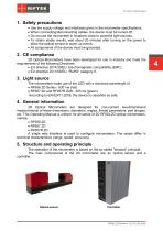
Use the supply voltage and interfaces given in the micrometer specifications. When connecting/disconnecting cables, the device must be turned off. Do not use the micrometer in locations close to powerful light sources. To obtain stable results, wait about 20 minutes after turning on the power to allow the optical sensor to warm up evenly. · All components of the device must be grounded. 2. CE сompliance 2D Optical Micrometers have been developed for use in industry and meet the requirements of the following Directives: · EU directive 2014/30/EU. Electromagnetic compatibility (EMC). · EU directive...

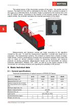
The optical sensor of the micrometer consists of two parts - the emitter and the receiver. The light from the LED is collimated by the lens. When a product is placed in the region of a collimated beam, its shadow image is projected by the receiver lens onto the 2D CMOS sensor. According to the location of the shadow border of the image (object profile), the controller calculates the required parameters of the object. Measurements and tolerance control are made according to the algorithm created by the user. To build the measurement algorithm, a simple and visual tool is proposed - the measurement...

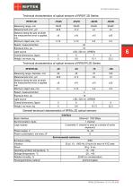
Technical characteristics of optical sensors of RF657.2D Series: RF657.2D Measuring range, mm Measurement error, µm Distance along the axis at which the measurement error is applied, mm Minimum object size, mm Speed, measurements/s Light source Overall dimensions, figure Technical characteristics of optical sensors of RF657R.2D Series: RF657R.2D Measuring range, diameter, mm Measurement error, µm Distance along the axis at which the measurement error is applied, mm Minimum object size, mm Speed, measurements/s Light source Overall dimensions, figure General technical characteristics of RF65x.2D...

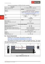
Technical characteristics of RF65x.2D-SuM controllers: Parameter Speed, measurements/s 3 x GbE, RJ-45 connectors 4 x RS-232/422/485, DB-9 connectors. Changing the interface type can be done in the BIOS (see Annex 2. Configuring the protocol for controller serial interfaces). 2 x RS-232, RJ-45 connectors 4 x USB 3.2 Gen 2 (10 6 x USB 3.2 Gen 2 (10 Gb/s) Gb/s) 2 x USB 2.0 1 x HDMI 1 x DisplayPort Power Power supply, V Power consumption, not more, W Standard 12...24 60 AT/ATX, switchable Environmental resistance Operating ambient temperature, °С Storage temperature, °С Permissible relative humidity...

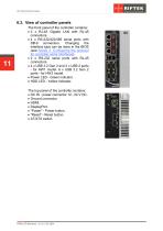
6.3. View of controller panels The front panel of the controller contains: · 3 x RJ-45 Gigabit LAN with RJ-45 connectors. · 4 x RS-232/422/485 serial ports with DB-9 connectors. Changing the interface type can be done in the BIOS (see Annex 2. Configuring the protocol for controller serial interfaces). · 2 x RS-232 serial ports with RJ-45 connectors. · 4 x USB 3.2 Gen 2 and 2 x USB 2 ports - for HW1 model, 6 x USB 3.2 Gen 2 ports - for HW2 model. · Power LED - Green indicator. · HDD LED - Yellow indicator. The top panel of the controller contains: · DC IN - power connector 12...24 V DC. · Ground...

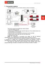
7. Connection options The block diagram of the connection options is shown in the figure. The red box shows the standard set, which includes: · Controller RF656.2D SuM. · Optical sensor RF656.2D of the required range (up to four optical sensors can be connected to one controller). · Ethernet cable for connecting the optical sensor to the controller. · Optical sensor power cable with sync and output lines. · Controller power cable. NOTE. Pin assignment of connectors and cables, as well as electrical characteristics of the inputs/outputs of the optical sensor are shown in Annex 1. The green box...

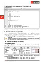
8. Example of item designation when ordering RF656.2D-R-LP-LS-LI Symbol Description x 6 or 7 or 7R R Measuring range of the optical sensor. RF656.2D-(FOV, height x width, mm): · 8x10 · 25x30 · 30x40 · 40x50 RF657.2D-(FOV, height x width, mm): · 15x20 · 25x35 · 40x50 · 60x80 RF657R.2D-(FOV, diameter, mm): · 25 · 45 · 70 · 100 LP The length of the controller power cable, m. LS The length of the power and sync cable of the optical sensor, m. LI The length of the Ethernet cable, m (max. 100). Example: RF656.2D-40x50-3-3-10 - optical sensor with measuring range 40x50 mm, controller power cable length...

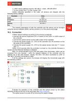
· LAN3: device address must be 192.168.2.*, mask - 255.255.255.0 (* is any number from 1 to 254, except 130) Unless otherwise specified in the order, all sensors are shipped with the following factory settings: Parameter mode Value static The network parameters of both the controller and the sensor can be changed using the service software (SDK), service protocol, or on the device web page. 10.2. Connection  Make network settings according to the previous paragraph.  Connect the service equipment (PC or switch) to the LAN1 or LAN3 output of the controller.  Connect the optical sensor to the...

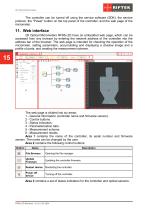
The controller can be turned off using the service software (SDK), the service protocol, the "Power" button on the top panel of the controller, and the web page of the micrometer. 11. Web interface 2D Optical Micrometers RF65x.2D have an embedded web page, which can be accessed from any browser by entering the network address of the controller into the address bar of the browser. The web page is intended for checking the operation of the micrometer, setting parameters, accumulating and displaying a shadow image and a profile of parts, and creating the measurement scheme. The web page is divided...

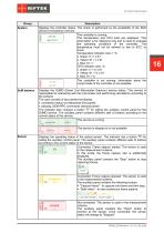
Group System Description Displays the controller status. The check is performed by the availability of the SUD (Smart Unit Daemon) service. The controller is running. The temperature and CPU load are displayed. This information is for reference only and is used to evaluate the operating conditions of the controller. The temperature must not be allowed to rise to 90°C or more. Temperature indicator color, t °C: · Green: 0 < t 61 · Yellow: 61 < t 91 · Red: 91 < t CPU indicator color, %: · Green: 0 < % 61 · Yellow: 61 < % 91 · Red: 91 < % The controller is not running. Information about the current...