Catalogs >
Imagine Optic >
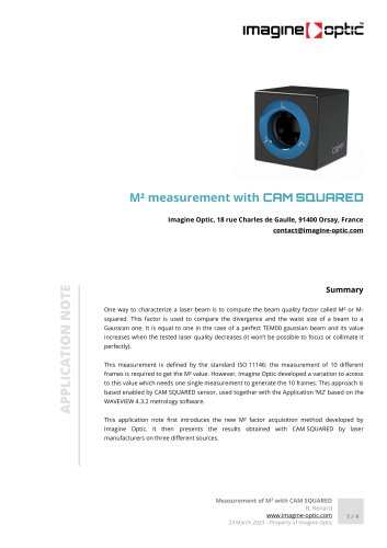
Calculation of beam parameters from local slopes - VIS NIR optical metrology Application Notes

Calculation of beam parameters from local slopes - VIS NIR optical metrology Application Notes
4Pages

Catalog excerpts

Calculation of beam parameters from local slopes - VIS NIR optical metrology Application Notes - 1

Calculation of beam parameters from local slopes Imagine Optic, 18 rue Charles de Gaulle, 91400 Orsay, France contact@imagine-optic.com When a light wave passes through an optical system, we can consider a phase shift function ݜ corresponding to the difference between the theoretical perfect wavefront and the one carrying the optical defects of the system. Ѱݜ is equal to zero if the system is perfect. In case of a circular pupil, these phase differences can be approximated by projecting the phase map onto the orthogonal basis of Zernike polynomials, the elements that describe wavefront aberrations. Calculation of beam parameters from local slopes Application note www.imagine-optic.com 25 February 2022 Ѣ Property of Imagine Optic

Open the catalog to page 1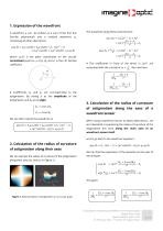

Calculation of beam parameters from local slopes - VIS NIR optical metrology Application Notes - 2

1. Expression of the wavefront A wavefront ݜ can be written as a sum of the first five Zernike The wavelines along these axes become: containing all other aberrations: ߰ݜ(Ѱݜ, ̰ݜ) = ðݑ1 Ͱݜ cos(̎) + ذݑ2 Ͱݜ sin(̎) + ذݑ3 ͢˅ (2ݜ2 ̢Ȓ 1) + ݑ4 Ͱݜ2 cos(2̎) + ذݑ5 Ͱݜ2 sin(2̎) + ذݜ Ѱݑ (߰ݜ, ̰ݜ) where (߰ݜ, ̰ݜ) is the polar coordinates on the circular normalized pupil (i.e. ðݜ ̢Ȉ [0; 1]), and ݑ Ͱݑ is the i-th Zernike coefficient. ֢׏ The coefficients in front of the terms in (ݜ̰ݑ)2 are associated with the curvature 2߰ݛ = 3. Calculation of the radius of curvature of astigmatism along the axes of a wavefront...

Open the catalog to page 2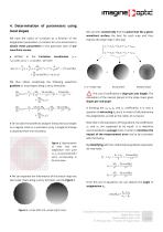

Calculation of beam parameters from local slopes - VIS NIR optical metrology Application Notes - 3

4. Determination of parameters using local slopes We can then numerically find the plane that fits a given We have the radius of curvature as a function of the astigmatism parameters. It remains for us to know how to wavefront surface the best for each map and thus express the slope map in this way: obtain these parameters in the particular case of our Űݑ߰ݜ cos(̎) ذݑΰݑ۰ݑ Ѱݑ = ưݑ߰ݜ sin(̰ݜ)), we have: Ï(ưݑ, Űݑ) = We thus obtain analytically the following wavefront gradient or local slopes along x and y directions: ߰ݜհݜ Ѱݑ1 4Ͱݑ3 2Ͱݐ cos 2԰ݜ0 2ðݐ sin 2԰ݜ0 (ðݑ, Űݑ) = +( + ) ưݑ+ Űݑ ưݜհݑ Űݑ ߰ݑ߂...

Open the catalog to page 3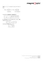

Calculation of beam parameters from local slopes - VIS NIR optical metrology Application Notes - 4

Note If ݑ ΰݑ = Űݑ ϰݑ , it is necessary to look at the value of ưݑϰݑ + Űݑ ΰݑ 2 We deduce the amplitude of astigmatism аݐ: 2 And finally the Focus coefficient ưݑ3 is Ͱݑ3 =

Open the catalog to page 4